
Have you ever wondered what the difference is between an AI developer with 10 years of experience who has a low-paying, dead-end job and a FANG AI engineer earning $100K with stock options and getting promoted to team leader next month?
Table of Contents
What Makes the Difference?
The difference lies in what one knows; the person with dead-end and low-pay jobs just knows how to use models on HungFace, and the developer on the opposite spectrum knows the ins and outs of complex AI architectures like CNNs.
This blog is for those who want to understand the algorithms just like a top Expert, for securing the dream job or making an impact on the world.
This is part 2 of from Master CNN like a Top Expert, if you are new, I would recommend that you read Part 1 Master CNN like Top Expert, Even if You Terrible at Maths first and comback on this.
A quick recap of what we’ve covered so far:
Part 1:
- What exactly are CNNs
- Explanation of how CNNs work
- Different layers and how they function
- The basic mathematics of CNNs
- The basic mathematics of each layer
In this blog, you will learn:
- Basics of NumPy
- Handling Images in NumPy
- Creating all The Layers in NumPy from Scratch
Basics of NumPy
Before we build a Convolutional Neural Network (CNN) from scratch, we need to master the one tool every top AI expert uses daily: NumPy.
Think of NumPy as the bedrock of AI programming in Python. While libraries like PyTorch and TensorFlow steal the spotlight, underneath, they all rely on NumPy-like tensor operations. So if you can master NumPy, you’re halfway to mastering deep learning.
Let’s start with the essentials:
1. What is NumPy?
NumPy (short for Numerical Python) is a high-performance library for numerical computing. It gives you:
- ndarrays (N-dimensional arrays) that are faster and more powerful than Python lists
- Vectorized operations (no for-loops!)
- Matrix multiplication, dot products, reshaping, slicing, and all the tools needed to handle image data like a pro
NumPy Intro
NumPy (Numerical Python) is the foundation for scientific computing in Python. It provides support for large, multi-dimensional arrays and matrices, along with a collection of mathematical functions to operate on them. It’s fast, thanks to its implementation in C, and is a must-know for AI developers working with data.
Getting Started
To use NumPy, first install it using pip if you haven’t already: pip install numpy. Then, import it in your Python script:
import numpy as npCreating Arrays
NumPy arrays are the core of the library. You can create them from Python lists or use built-in functions:
# From a list
arr = np.array([1, 2, 3, 4])

# 2D array
arr_2d = np.array([[1, 2], [3, 4]])

# Using built-in functions
zeros = np.zeros((2, 3))  # 2x3 array of zeros
ones = np.ones((3, 2))    # 3x2 array of ones
arange = np.arange(0, 10, 2)  # Array from 0 to 9, step 2: [0, 2, 4, 6, 8]
Array Indexing
Access elements in a NumPy array using indices, similar to Python lists:
arr = np.array([10, 20, 30, 40])
print(arr[1])  # Output: 20

# 2D array indexing
arr_2d = np.array([[1, 2], [3, 4]])
print(arr_2d[1, 0])  # Output: 3
Array Slicing
Slicing extracts a portion of the array. Use the syntax arr[start:end:step]:
arr = np.array([0, 1, 2, 3, 4, 5])
print(arr[1:4])  # Output: [1, 2, 3]

# 2D slicing
arr_2d = np.array([[1, 2, 3], [4, 5, 6]])
print(arr_2d[0, 1:3])  # Output: [2, 3]
Data Types
NumPy arrays have specific data types (e.g., int32, float64). You can check or set the type:
arr = np.array([1, 2, 3])
print(arr.dtype)  # Output: int64 (or int32 depending on system)

# Specify type
arr_float = np.array([1, 2, 3], dtype='float32')
print(arr_float.dtype)  # Output: float32
Copy vs View
A copy creates a new array, while a view references the original array:
arr = np.array([1, 2, 3])
copy_arr = arr.copy()  # Independent copy
view_arr = arr.view()  # View of the original

copy_arr[0] = 10
print(arr)  # Output: [1, 2, 3]

view_arr[0] = 10
print(arr)  # Output: [10, 2, 3]
Array Shape
The shape of an array is its dimensions:
arr = np.array([[1, 2, 3], [4, 5, 6]])
print(arr.shape)  # Output: (2, 3) - 2 rows, 3 columns
Array Reshape
Reshape changes the array’s dimensions without altering its data:
arr = np.array([1, 2, 3, 4, 5, 6])
reshaped = arr.reshape(2, 3)
print(reshaped)  # Output: [[1, 2, 3], [4, 5, 6]]
Array Iterating
Iterate over arrays using loops or NumPy’s nditer for efficiency:
arr = np.array([[1, 2], [3, 4]])
for x in np.nditer(arr):
    print(x, end=' ')  # Output: 1 2 3 4
Array Join
Combine arrays using functions like concatenate, stack, or hstack:
arr1 = np.array([1, 2])
arr2 = np.array([3, 4])
joined = np.concatenate((arr1, arr2))
print(joined)  # Output: [1, 2, 3, 4]
Array Split
Split an array into multiple sub-arrays:
arr = np.array([1, 2, 3, 4, 5, 6])
split_arr = np.array_split(arr, 3)
print(split_arr)  # Output: [array([1, 2]), array([3, 4]), array([5, 6])]
Array Search
Find indices where a condition is met using where:
arr = np.array([10, 20, 30, 20])
indices = np.where(arr == 20)
print(indices)  # Output: (array([1, 3]),)
Array Sort
Sort arrays with sort:
arr = np.array([3, 1, 4, 2])
sorted_arr = np.sort(arr)
print(sorted_arr)  # Output: [1, 2, 3, 4]
Array Filter
Filter arrays using boolean indexing:
arr = np.array([1, 2, 3, 4])
filter_arr = arr > 2
filtered = arr[filter_arr]
print(filtered)  # Output: [3, 4]
Mastering these NumPy basics will set a strong foundation for building and manipulating CNN layers in the upcoming sections.
Handling Images in NumPy
Now that you’ve got the basics of NumPy under your belt, let’s move on to something more exciting: handling images! In CNNs, images are the primary input, and NumPy is your go-to tool for loading, manipulating, and preprocessing them before feeding them into your model. Let’s break this down step by step.
Loading an Image as a NumPy Array
Images are essentially arrays of pixel values, and NumPy is perfect for working with them. To load an image, you’ll need a library like Pillow (PIL) or imageio to read the image file and convert it into a NumPy array. Here’s how you can do it with Pillow:
from PIL import Image
import numpy as np

# Load the image
image = Image.open("example.jpg")  # Replace with your image path
image_array = np.array(image)

print(image_array.shape)  # Output: (height, width, channels), e.g., (224, 224, 3) for an RGB image

The resulting array has a shape of (height, width, channels), where channels is typically 3 for RGB images (red, green, blue) or 1 for grayscale.
Visualizing the Image
To check your work, you can visualize the modified image using a library like matplotlib:
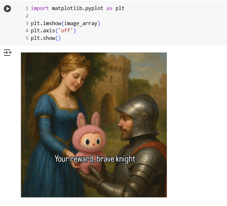
import matplotlib.pyplot as plt

plt.imshow(image_array)
plt.axis('off')
plt.show()
This will display the image, helping you verify that your preprocessing steps are working as expected.
Converting to Grayscale
Color images can be computationally heavy, so you might want to convert them to grayscale for simpler processing. Here’s how:
# Convert to grayscale
gray_image = np.mean(image_array, axis=2).astype(np.uint8)  # Average across the channel axis
print(gray_image.shape)  # Output: (height, width), e.g., (224, 224)
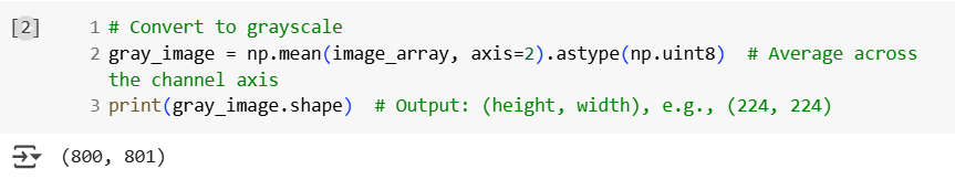
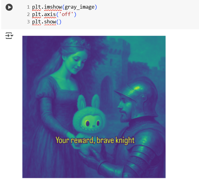
This reduces the image to a 2D array, where each value represents the intensity of the pixel (0 to 255).
Normalizing Pixel Values
CNNs often perform better when pixel values are normalized to a range like [0, 1] or [-1, 1]. Since pixel values in images are typically between 0 and 255, you can normalize them easily:
normalized_image = image_array / 255.0
print(normalized_image.min(), normalized_image.max())  # Output: 0.0 1.0
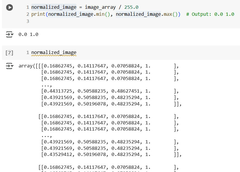

This step is crucial for training your CNN, as it ensures all input values are on a consistent scale.
Now I would like you all to print the images yourselves to encourage practice—not because I’m too lazy to include them in every code block.
Resizing Images
Images often come in different sizes, but CNNs typically require a fixed input size (e.g., 224×224 for many models). You can resize images using libraries like Pillow and then convert them back to a NumPy array:
# Resize the image
resized_image = image.resize((224, 224))  # Resize to 224x224
resized_array = np.array(resized_image)

print(resized_array.shape)  # Output: (224, 224, 3)
Cropping and Padding
Sometimes, you need to crop or pad images to focus on specific regions or match a required size. NumPy makes this straightforward:
# Cropping
cropped_array = image_array Strong style[50:150, 50:150, :]  # Crop a 100x100 section
print(cropped_array.shape)  # Output: (100, 100, 3)

# Padding (e.g., to add a border of zeros)
padded_array = np.pad(image_array, ((10, 10), (10, 10), (0, 0)), mode='constant', constant_values=0)
print(padded_array.shape)  # Output: (height+20, width+20, 3)
Flipping and Rotating
Data augmentation—like flipping or rotating images—can help improve your CNN’s performance by increasing the variety of training data:
# Flip vertically
flipped_vertical = np.flipud(image_array)

# Flip horizontally
flipped_horizontal = np.fliplr(image_array)

# Rotate 90 degrees
rotated = np.rot90(image_array)
Accessing and Modifying Pixel Values
You can directly manipulate pixel values using NumPy’s indexing. For example, let’s brighten an image by increasing pixel values:
brightened_image = np.clip(image_array + 50, 0, 255) # Add 50 to all pixels, clip to valid range
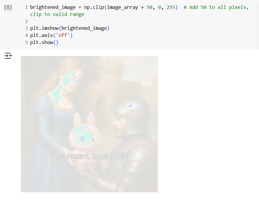
This is useful for experimenting with image preprocessing techniques that can enhance your CNN’s ability to learn.
Now let’s get started with the more fun stuff—creating different layers of a CNN on our own.
Walking Through the Layers
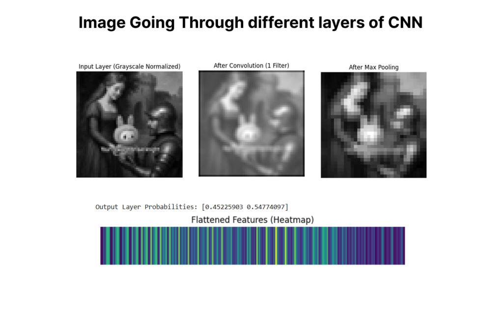
Input Layer
The input_layer function loads example.jpg, resizes it to 64×64 pixels, converts it to grayscale (to simplify processing), and normalizes the pixel values to [0, 1]. The output is a 2D array of shape (64, 64). This preprocessing ensures the image is in a format suitable for the CNN.
def input_layer(image_path, target_size=(64, 64)):
    """
    Loads an image, converts to grayscale, resizes, and normalizes it.
    Args:
        image_path (str): Path to the image file.
        target_size (tuple): Desired (height, width) for resizing.
    Returns:
        np.ndarray: Preprocessed image array of shape (height, width).
    """
    # Load the image
    image = Image.open(image_path)
    # Resize to target size
    image = image.resize(target_size)
    # Convert to NumPy array
    image_array = np.array(image)
    # Convert to grayscale
    if len(image_array.shape) == 3:  # If RGB, convert to grayscale
        image_array = np.mean(image_array, axis=2).astype(np.uint8)
    # Normalize to [0, 1]
    image_array = image_array / 255.0
    return image_array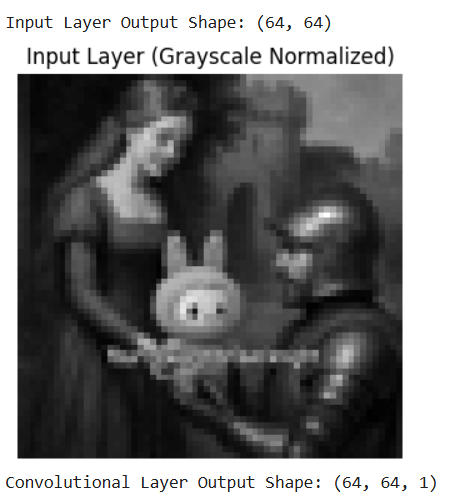
Convolutional Layer
The convolutional_layer function applies convolution using a 3×3 kernel (a simple averaging filter for this example). We use padding=’same’, which adds a 1-pixel border of zeros around the input (since (3-1)/2 = 1) to ensure the output spatial dimensions match the input (64×64). The stride is 1, and we use 1 filter, so the output shape is (64, 64, 1). The convolution operation slides the kernel over the image, computing the weighted sum at each position to extract features like edges or textures.
def convolutional_layer(input_data, kernel_size=3, num_filters=1, stride=1, padding='same'):
    """
    Applies convolution to the input with specified kernel size, filters, stride, and padding.
    Args:
        input_data (np.ndarray): Input array of shape (height, width).
        kernel_size (int): Size of the kernel (e.g., 3 for 3x3).
        num_filters (int): Number of filters to apply.
        stride (int): Step size for convolution.
        padding (str): 'same' to add padding, 'valid' for no padding.
    Returns:
        np.ndarray: Convolved output of shape (out_height, out_width, num_filters).
    """
    height, width = input_data.shape
    kernel = np.ones((kernel_size, kernel_size)) / (kernel_size * kernel_size)  # Simple averaging kernel

    # Calculate padding
    if padding == 'same':
        pad_size = (kernel_size - 1) // 2
        input_padded = np.pad(input_data, ((pad_size, pad_size), (pad_size, pad_size)), mode='constant', constant_values=0)
    else:
        input_padded = input_data
        pad_size = 0

    # Calculate output dimensions
    out_height = (height + 2 * pad_size - kernel_size) // stride + 1
    out_width = (width + 2 * pad_size - kernel_size) // stride + 1
    output = np.zeros((out_height, out_width, num_filters))

    # Apply convolution for each filter
    for f in range(num_filters):
        for i in range(0, out_height):
            for j in range(0, out_width):
                region = input_padded[i*stride:i*stride+kernel_size, j*stride:j*stride+kernel_size]
                output[i, j, f] = np.sum(region * kernel)

    return output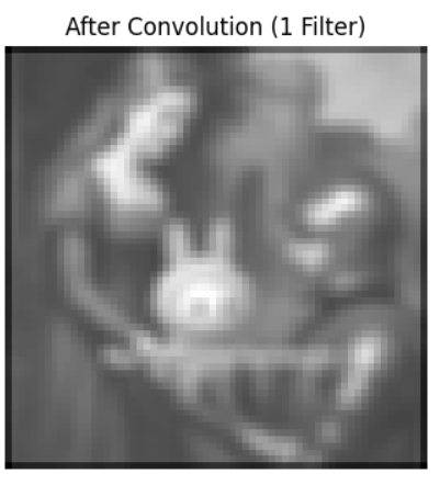
Pooling Layer
The pooling_layer function applies max pooling with a 2×2 window and a stride of 2. This reduces the spatial dimensions by half: from (64, 64, 1) to (32, 32, 1). Max pooling takes the maximum value in each 2×2 region, which helps reduce computational complexity and makes the model more robust to small translations in the image.
def pooling_layer(input_data, pool_size=2, stride=2, pool_type='max'):
    """
    Applies pooling to the input to reduce spatial dimensions.
    Args:
        input_data (np.ndarray): Input array of shape (height, width, channels).
        pool_size (int): Size of the pooling window (e.g., 2 for 2x2).
        stride (int): Step size for pooling.
        pool_type (str): 'max' for max pooling, 'avg' for average pooling.
    Returns:
        np.ndarray: Pooled output of shape (out_height, out_width, channels).
    """
    height, width, channels = input_data.shape
    out_height = (height - pool_size) // stride + 1
    out_width = (width - pool_size) // stride + 1
    output = np.zeros((out_height, out_width, channels))

    for c in range(channels):
        for i in range(out_height):
            for j in range(out_width):
                region = input_data[i*stride:i*stride+pool_size, j*stride:j*stride+pool_size, c]
                if pool_type == 'max':
                    output[i, j, c] = np.max(region)
                elif pool_type == 'avg':
                    output[i, j, c] = np.mean(region)

    return output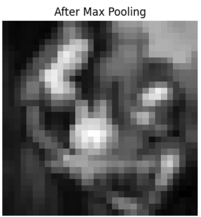
Output Layer
The output_layer function flattens the pooling output (from (32, 32, 1) to a 1D array of size 32*32*1=1024) and applies a fully connected layer. We simulate a binary classification task (2 classes) by using random weights and biases to compute logits, then apply the softmax function to get probabilities. The output is a 1D array of shape (2,), representing the probability of each class.
def output_layer(input_data, num_classes=2):
    """
    Flattens the input and applies a fully connected layer for classification.
    Args:
        input_data (np.ndarray): Input array of shape (height, width, channels).
        num_classes (int): Number of output classes.
    Returns:
        np.ndarray: Output probabilities of shape (num_classes,).
    """
    # Flatten the input
    flattened = input_data.flatten()
    # Simulate a fully connected layer with random weights
    weights = np.random.randn(flattened.size, num_classes) * 0.01  # Small random weights
    biases = np.zeros(num_classes)
    # Compute output (logits)
    logits = np.dot(flattened, weights) + biases
    # Apply softmax to get probabilities
    exp_logits = np.exp(logits)
    probabilities = exp_logits / np.sum(exp_logits)
    return probabilities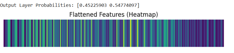
So, to sum it up and get some image SEO juice, here’s an image capturing the evolution of an image as it passes through all the CNN layers. It’s fascinating how, with each layer, we lose some visual quality but gain deeper insight about the image. It goes to show that sometimes, you must break things down in order to build something greater.
Until we meet again
In the next Blog we will be coding whole CNN from just Numpy stay tuned, and for updates follow me on x
Amarnath Pandey
Leave a Reply