Master CNN like Top Expert, Even if You Terrible at Maths

If you are a deep learning engineer or researcher, it’s nearly impossible not to have heard of CNNs (Convolutional Neural Networks). They are one of the most widely used AI architectures in the modern AI development landscape.

In this blog, part 1 of 3, I will explain how you can create incredibly useful, production-level CNN models and touch on VLMs, a more modern evolution of CNNs.

Here’s what you’ll learn in this blog:

• An Introduction to CNNs
• Understanding Different Types of Layers in CNNs and How They Work
• A Complete Mathematical Breakdown of Every Equation That Scares You

Introduction to CNN

CNN is a computer algorithm that was created by Yann LeCun, a French-American computer scientist. CNN is a type of ANN (Artificial Neural Network) that specializes in image classification.

A cool fact: Yann LeCun is currently the Chief Scientist at Meta AI. How amazing is that—the father of CNN is now building AI projects at Meta! LOL 🙂

Now, back to the topic. To understand how a CNN works, we’ll be exploring the mathematics behind it, writing code from scratch, and using PyTorch.

Prerequisites

Requirement	Description
Python Programming	Comfortable with functions, loops, and data structures
Algebra & Statistics	Variables, equations, mean, median, standard deviation
Basic Machine Learning Concepts	Understanding of supervised learning and datasets
NumPy & Pandas (Recommended)	Experience with arrays and dataframes for data manipulation
Computing Environment	Python, Jupyter/Colab, and (optionally) a GPU for faster training

Dataset Overview

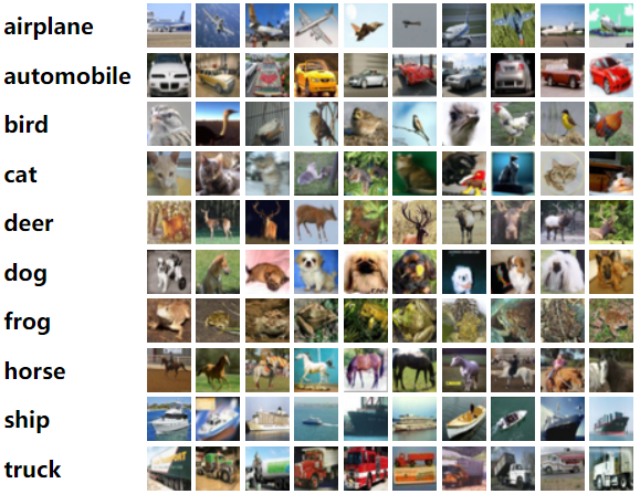
In this blog, I’m going to use the CIFAR-10 dataset-a widely recognized benchmark in the field of computer vision and machine learning. CIFAR-10 consists of 60,000 color images, each sized at 32×32 pixels, and these images are evenly divided into 10 different classes. 

Each class contains 6,000 images, with 50,000 images dedicated to training and 10,000 reserved for testing.

The reason I chose CIFAR-10 is its popularity and relevance for image classification tasks.

The diversity and structure of CIFAR-10 have made it a standard for evaluating new algorithms and comparing model performance across the research community.

What Does Each Layer of the Network Do?

Below, I’ve shared GIFs from a very popular website called CNN Explainer. This is something I’ve recommended to almost everyone who wanted to learn about Convolutional Neural Networks (CNNs). If you’re serious about learning computer vision, this is one of the best resources out there.

Input layer

The input layer is the entry point of a Convolutional Neural Network (CNN). For image data, this layer simply receives the raw pixel values of the image. For example, in the case of the CIFAR-10 dataset, each input is a 32×32×3 array, representing the width, height, and three color channels (RGB) of the image. The input layer does not perform any computation or transformation; it just passes the data to the next layer in the network.

Convolutional Layers

Convolution in CNNs means sliding a small filter (kernel) over the input image and, at each position, computing a weighted sum of the input pixels covered by the filter. The weights are the values in the filter.

Step-by-Step Breakdown

1. Sliding the Filter
   • Imagine your input image as a stack of 2D grids (one for each color channel).
   • The filter is a smaller stack of grids, with the same number of channels.
   • You place the filter at the top-left corner of the input and “slide” it across the image, one step at a time (this step is called the stride).

Pooling layer

A Pooling layer is used to reduce the spatial dimensions (width and height) of feature maps, making the network more efficient. It works by sliding a window over the input and taking the maximum or average value within that window (e.g., Max Pooling or Average Pooling). This helps retain important features while reducing computation and preventing overfitting.

Output Layer

The output layer in a Convolutional Neural Network (CNN) is the final stage where the model makes its predictions. After the convolutional layers have extracted and processed features, the output layer applies a function—typically softmax for classification tasks, to convert raw scores (logits) into probabilities.

Each node in the output layer corresponds to a class label; for example, in the CIFAR-10 dataset, the output layer has 10 neurons, each representing a different image category (like cat, airplane, or truck). The class with the highest probability is selected as the model’s prediction.

Breaking Down the Mathematics Behind CNN Models

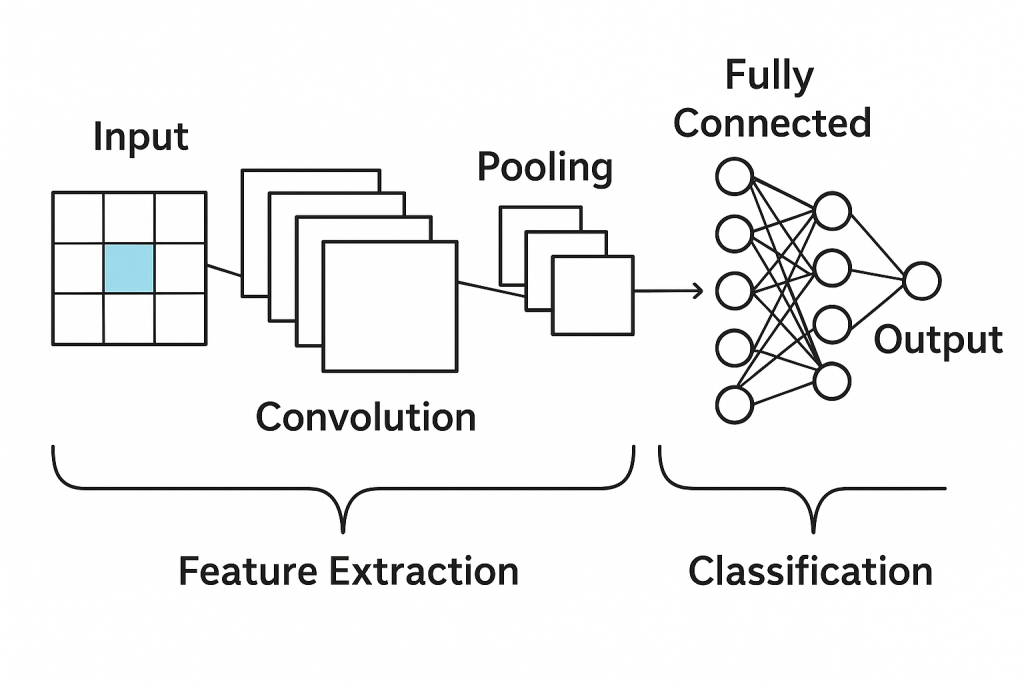
The CNN model has the following two parts :

1. Feature Learning
2. Classification

Hear, I have attached a very important video that you should watch. It presents a hypothesis on how CNNs might learn the patterns they learn.

Feature Learning

At the heart of CNNs lies the idea of automatically learning patterns from input images. Unlike traditional machine learning, where you manually extract features like edges or textures, CNNs learn them through layers—specifically convolution, activation, and pooling layers.

Let’s understand how each part works.

Convolution Layer – Extracting Raw Features

Imagine you have a small flashlight and you’re scanning a big photo—one patch at a time. At each patch, you’re asking: “Does this part look like something meaningful?”

That flashlight is called a kernel or filter—a small grid of numbers (like 3×3 or 5×5). You slide it over the image and at every position, multiply the overlapping values and add them up.

Mathematically:

f[i,j] = \sum_{x=1}^{m_1} \sum_{y=1}^{m_2} \sum_{z=1}^{m_c} K[x, y, z] \cdot I[i + x – 1, j + y – 1, z]

This equation means:

• Take a patch of the image (I) starting at position (i,j)(i, j)
• Multiply each value in the kernel K with the matching value in that patch
• Add them all up → This gives one number in the output at (i,j)(i, j)

Here’s how you calculate a single pixel, say f[1,1]:

f[1,1] = \sum_{x=-2}^{2} \sum_{y=-2}^{2} K[x,y] \cdot I[1 – x, 1 – y]

Let’s break that down:

• You’re using a 5×5 kernel (range: -2 to 2)
• You “flip” the kernel (which is why the formula is 1−x1 – x1−x and 1−y1 – y1−y)
• You apply it centered at image location (1,1)

Now apply the formula to a real image and kernel (example below), substitute zeros where values fall outside the image (common practice called zero-padding):

f[1,1] = K[-2,-2] \cdot I[3,3] + K[-1,-2] \cdot I[2,3] + \dots + K[2,2] \cdot I[-1,-1]

Since many indices like [−1,−1] or [0,3] are invalid (they fall outside the image), they get replaced by 0.

Now plug in values:
f[1,1] = 0 + 0 + 0 + 0 + 0 + (1 \cdot 1) + (0 \cdot 1) + (1 \cdot 0) + (0 \cdot 1) + 0 + \dots + (1 \cdot 1) = 3

This value now represents the strength of the pattern the kernel is looking for at position (1,1).

Padding – Preserving the Edges

The problem with convolution is that when the kernel slides over the image, it can’t align fully at the borders. So your output shrinks.

To fix this, we pad the image with zeros around the border. Padding lets you keep the output size the same as the input or control it exactly.

Here’s how padding helps calculate a single pixel at the edge:
Padding ensures that even when the kernel is centered on a corner or border pixel, it has enough “context” (i.e., values, even if zeros) to compute that output. Without padding, those positions would be skipped or truncated.

Bias and Activation – Adding Non-Linearity

After convolution, we don’t stop there. We apply a bias term to the result to give the network more flexibility.

c = f[i,j] + b

This just adds a small number to the output. Then we apply an activation function, typically ReLU:
R(x) = \max(0, x)

This function zeroes out all negative values.

Here’s how you calculate a single pixel after activation:

• Compute the convolution at pixel (i,j)(i, j)(i,j)
• Add the bias bbb
• Apply the ReLU function: if the result is negative, make it zero; if it’s positive, keep it

Example:

f[i,j] = -2 \Rightarrow R(f[i,j]) = 0 \quad \text{or} \quad f[i,j] = 12 \Rightarrow R(f[i,j]) = 12

This step ensures that only strong, positive responses survive in the next layer.

---

Pooling Layer – Shrinking the Feature Map

Even after activation, the output feature map can still be large. Pooling helps by reducing its size, summarizing nearby values.

In max pooling, we take the maximum value from each small region (typically 2×2 or 3×3).

Here’s how you calculate a single pixel after pooling:
Take a small patch of the activated feature map (say 2×2), and pick the highest number in that patch. That maximum value becomes a single pixel in the pooled output.

Example:

From a 2×2 region:

1 4  
2 3

You take the maximum:

max(1,4,2,3)=4

This output becomes the value at one pixel in the downsampled feature map.

Pooling Output Size:

The size of the pooled output is calculated as:

\text{dim of pooled output } P = \left( \frac{sm_1 + 2p – n_1}{s} \right) \times \left( \frac{sm_2 + 2p – n_2}{s} \right) \times m_c
Where:

Where:
m_1, m_2\,: \text{ input image dimensions}
n_1, n_2\,: \text{ size of pooling window}
p\,: \text{ padding}
s\,: \text{ stride}
m_c\,: \text{ number of channels (unchanged)}

This formula tells you how many pixels you’ll get after pooling.

2. Classification in Convolutional Neural Networks

Once a CNN finishes learning features through convolution, activation, and pooling, we arrive at the final step: Classification.

This part is where the network takes everything it has learned—edges, textures, shapes—and decides what the image actually represents. Is it a cat? A car? A banana?

To do this, CNNs use one or more Fully Connected Layers at the end.

Fully Connected Layer – Making the Final Decision

All the extracted features—now condensed through pooling—are laid out in a single line. This process is called flattening.

Flattening

If your final pooled feature map looks like this:

4  3  
4  3

Flattening simply turns it into a 1D array (vector):

[4, 3, 4, 3]

This flattened vector is then passed to the fully connected layer.

What does the Fully Connected Layer do?

Think of it like a traditional neural network. Each number in the flattened vector is connected to a neuron. These neurons compute a weighted sum of all the values, add a bias, and apply an activation function.

Mathematically:

X = \sum_i w_i P_i + b’ \
z = g(X)

P_i \text{ is the } i\text{-th element in the flattened vector (our pooled features)}
w_i \text{ is the weight assigned to each input}
b’ \text{ is the bias}
g \text{ is an activation function (like ReLU, sigmoid, or softmax)}

Here’s how you calculate a single pixel (neuron output) in the classification layer:

Let’s say your flattened feature vector is:

P = [4, 3, 4, 3]

And you want to calculate the output of one neuron in the fully connected layer. That neuron has:

• P \text{Weights: } [0.2, 0.5, -0.3, 0.1]
• \text{Bias: } b’ = 1.0

You multiply each input with its corresponding weight:

X = (4 \cdot 0.2) + (3 \cdot 0.5) + (4 \cdot -0.3) + (3 \cdot 0.1) + 1.0 = 0.8 + 1.5 – 1.2 + 0.3 + 1.0 = 2.4

Now apply an activation function, say ReLU:

z = \max(0, 2.4) = 2.4

That 2.4 is the neuron’s output—the activation value representing one possible class (or part of the decision for one).

If you’re classifying into multiple classes, you’ll have multiple neurons—one per class—and each will output a score. These scores are typically passed through a softmax function in the final layer to turn them into probabilities.

Softmax – Turning Outputs into Probabilities

The final layer often uses the softmax activation function, which takes the outputs from the neurons and turns them into probabilities that all add up to 1.

\text{softmax}(z_i) = \frac{e^{z_i}}{\sum_j e^{z_j}}

Where:

• z_i \text{: the score from neuron } i
• The denominator ensures all outputs are normalized into probabilities

For example, if the output layer gives:

[2.4, 1.0, 0.3]

After softmax, you might get:

[0.73,0.18,0.09]

This means the model is 73% confident in class 1, 18% in class 2, and 9% in class 3.

[End of Part 1]

Click Here to Read Part 2