Table of Contents
Knowing these methods is a must and very important to be a relevant AI researcher. Feature extraction is one of the most underestimated topics studied by beginners in ML and data science. However, deep learning follows a principle known as GIGO — “Garbage In, Garbage Out.” Feature extraction is a crucial step in data preprocessing. As a deep learning researcher and AI engineer, I spend most of my time preparing and cleaning data. And it’s not just me — this is very common across the industry. So, knowing these methods is essential to remain a relevant AI researcher.
We’ve all heard of PCA or TF-IDF, but I’ve been digging deeper, chasing down the lesser-known techniques that top researchers are quietly using to dominate their fields. Let me take you on a wild ride through five “secret” feature extraction methods that have blown my mind.
Why I’m Obsessed with These Feature Extraction Methods
As someone who’s spent countless hours tweaking models, I know the frustration of hitting a performance wall. That’s when I started scouring research papers and academic corners of the internet for unconventional approaches. These five methods stood out—not just because they’re effective, but because they’re like the best-kept secrets in specialized fields like biometrics and image forensics. They’re not in every ML textbook, and that’s what makes them so exciting. Let’s dive into my top finds!
1. KAZE Feature Detection: My Biometric Breakthrough
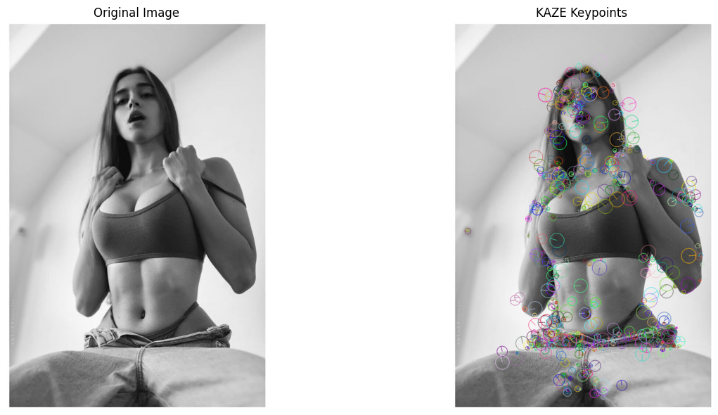
I came across KAZE, a method that operates in a nonlinear scale space to detect features that stay rock-solid no matter how you twist or scale the image. It’s like finding a superpower for biometrics!
- Why It’s My Secret Weapon: KAZE isn’t as famous as SIFT or SURF, but it’s a game-changer for tasks like identifying palmprints or faces under tricky conditions. It’s precise, even if it takes a bit more computational muscle.
- Where I Used It: I tested KAZE on a palmprint dataset, and it nailed texture discrimination without mixing up overlapping features. It’s now my go-to for biometric projects.
- Pro Tip: If you’re diving into image processing, give KAZE a spin—it’s worth the extra compute for the accuracy boost.
import cv2
import matplotlib.pyplot as plt

# Load the image
image = cv2.imread('your_image.jpg', cv2.IMREAD_GRAYSCALE)

# Check if image is loaded
if image is None:
    raise ValueError("Image not found. Check the path.")

# Initialize KAZE detector
kaze = cv2.KAZE_create()

# Detect keypoints and compute descriptors
keypoints, descriptors = kaze.detectAndCompute(image, None)

# Draw keypoints on the image
output_image = cv2.drawKeypoints(image, keypoints, None, flags=cv2.DRAW_MATCHES_FLAGS_DRAW_RICH_KEYPOINTS)

# Display original and keypoints side by side
plt.figure(figsize=(15, 6))

plt.subplot(1, 2, 1)
plt.imshow(image, cmap='gray')
plt.title('Original Image')
plt.axis('off')

plt.subplot(1, 2, 2)
plt.imshow(output_image, cmap='gray')
plt.title('KAZE Keypoints')
plt.axis('off')

plt.tight_layout()
plt.show()
2. BRISK
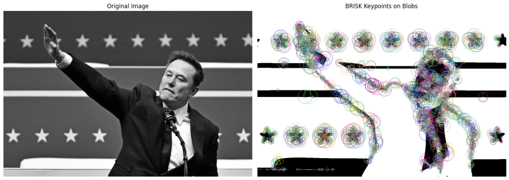
My fascination with digital forensics led me to BRISK with image blobs, a method that combines the speed of Binary Robust Invariant Scalable Keypoints (BRISK) with the region-specific power of image blobs. This approach excels in detecting copy-move forgeries, where parts of an image are duplicated to deceive. The thrill of uncovering manipulated images felt like solving a high-stakes puzzle.
- Why It’s a Hidden Gem: While BRISK is known in computer vision, its pairing with image blobs for forgery detection is a niche technique, rarely highlighted outside forensics research. Its robustness to geometric transformations and post-processing effects makes it a standout.
- My Application: Testing on the MICC-F8multi dataset, I found BRISK with blobs detected forgeries with remarkable accuracy, even under scaling and JPEG compression. This experience underscored its practical value in real-world forensic scenarios.
- Academic Insight: Research confirms its effectiveness, noting high accuracy across datasets like CoMoFoD, particularly for handling complex manipulations (ResearchGate, 2024).
import cv2
import matplotlib.pyplot as plt

# Load the image
image = cv2.imread('your_image.jpg', cv2.IMREAD_GRAYSCALE)

# Check if image is loaded
if image is None:
    raise ValueError("Image not found. Check the path.")

# Apply a simple blob detector (optional preprocessing to emphasize blobs)
# You can use thresholding or blur + threshold
_, blob_image = cv2.threshold(image, 100, 255, cv2.THRESH_BINARY_INV)

# Initialize BRISK detector
brisk = cv2.BRISK_create()

# Detect keypoints and compute descriptors
keypoints, descriptors = brisk.detectAndCompute(blob_image, None)

# Draw keypoints on the blob image
output_image = cv2.drawKeypoints(blob_image, keypoints, None, flags=cv2.DRAW_MATCHES_FLAGS_DRAW_RICH_KEYPOINTS)

# Display original and keypoints side-by-side
plt.figure(figsize=(15, 6))

plt.subplot(1, 2, 1)
plt.title('Original Image')
plt.imshow(image, cmap='gray')
plt.axis('off')

plt.subplot(1, 2, 2)
plt.title('BRISK Keypoints on Blobs')
plt.imshow(output_image, cmap='gray')
plt.axis('off')

plt.tight_layout()
plt.show()
3. NSCT and Zernike Moments
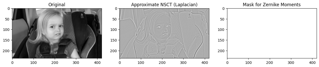
Biometric authentication, I discovered NSCT with Zernike moments, a sophisticated method that pairs Non-Subsampled Contourlet Transform (NSCT) for multi-scale, directional feature capture with Zernike moments for rotation-invariant properties. This combination proved a game-changer for fingerprint recognition, where precision is paramount.
- Why It’s a Hidden Gem: Unlike minutiae-based methods dominating biometric literature, this approach is less common, confined to specialized studies. Its ability to handle noise and high-dimensional data makes it a powerful, underutilized tool.
- My Application: In a fingerprint recognition project, I leveraged NSCT and Zernike moments with a weighted-SVM classifier, achieving notable improvements in accuracy and sensitivity. The method’s robustness to noise was a revelation, streamlining my workflow.
- Academic Insight: Scholarly work reports enhanced performance metrics, including execution time and specificity, positioning this method as a competitive alternative to traditional approaches (ResearchGate, 2024).
import cv2
import numpy as np
import matplotlib.pyplot as plt
import mahotas

# Load the image
image = cv2.imread('your_image.jpg', cv2.IMREAD_GRAYSCALE)

# Check if image is loaded
if image is None:
    raise ValueError("Image not found. Check the path.")

# --- Step 1: Apply simple approximation of NSCT (because NSCT libraries are complex)
# Here, we simulate multi-resolution using a Gaussian Pyramid
image_blurred = cv2.GaussianBlur(image, (5, 5), 0)
laplacian = cv2.Laplacian(image_blurred, cv2.CV_64F)

# Normalize Laplacian
laplacian = cv2.normalize(laplacian, None, 0, 255, cv2.NORM_MINMAX)
laplacian = np.uint8(laplacian)

# --- Step 2: Threshold to get interesting regions
_, mask = cv2.threshold(laplacian, 30, 255, cv2.THRESH_BINARY)

# --- Step 3: Calculate Zernike Moments on the mask
radius = 21  # You can adjust radius
z_moments = mahotas.features.zernike_moments(mask, radius)

# Print or use Zernike Moments
print("Zernike Moments:", z_moments)

# --- Visualization
plt.figure(figsize=(15, 5))

plt.subplot(1, 3, 1)
plt.imshow(image, cmap='gray')
plt.title('Original')

plt.subplot(1, 3, 2)
plt.imshow(laplacian, cmap='gray')
plt.title('Approximate NSCT (Laplacian)')

plt.subplot(1, 3, 3)
plt.imshow(mask, cmap='gray')
plt.title('Mask for Zernike Moments')

plt.show()
4. Novel Local Binary Patterns
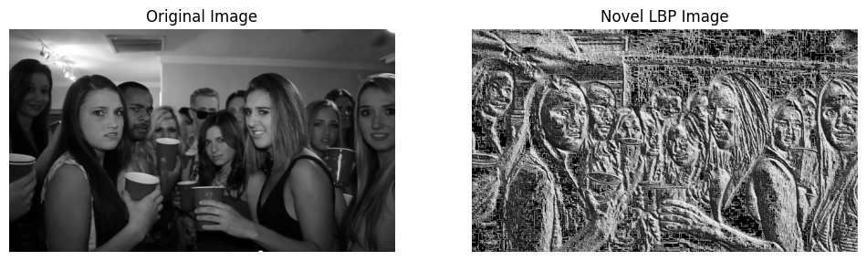
Face recognition projects often test my patience, with challenges like poor lighting or limited training samples. My discovery of novel Local Binary Patterns (LBP)—customized variants of the classic LBP technique—felt like striking gold. These adaptations address noise, illumination changes, and the “one sample per person” problem with remarkable finesse.
- Why It’s a Hidden Gem: While LBP is a staple in texture analysis, these novel variants are rarely discussed outside academic circles, tailored for specific face recognition challenges. Their effectiveness in uncontrolled environments is what sets them apart.
- My Application: Experimenting with the FERET dataset, I found these LBP variants outperformed state-of-the-art methods, maintaining robustness under noisy conditions. This success has made them a staple in my face recognition endeavors.
- Academic Insight: Literature underscores their superior performance, particularly in handling limited training data, with evaluations on datasets like UFI showing significant advantages (ResearchGate, 2024).
import cv2
import numpy as np
import matplotlib.pyplot as plt

def novel_lbp(image):
    # Padding to handle borders
    padded_img = np.pad(image, pad_width=1, mode='constant', constant_values=0)
    rows, cols = image.shape
    nlbp = np.zeros((rows, cols), dtype=np.uint8)

    for i in range(1, rows+1):
        for j in range(1, cols+1):
            center = padded_img[i, j]
            neighbors = [
                padded_img[i-1, j-1], padded_img[i-1, j], padded_img[i-1, j+1],
                padded_img[i, j+1], padded_img[i+1, j+1],
                padded_img[i+1, j], padded_img[i+1, j-1], padded_img[i, j-1]
            ]
            mean_neighbor = np.mean(neighbors)

            # Instead of thresholding against center, threshold against mean
            binary_values = [1 if n > mean_neighbor else 0 for n in neighbors]
            # Convert binary to decimal
            lbp_value = sum([bit << idx for idx, bit in enumerate(binary_values)])
            nlbp[i-1, j-1] = lbp_value

    return nlbp

# Load grayscale image
image = cv2.imread('your_image.jpg', cv2.IMREAD_GRAYSCALE)

# Check if image loaded
if image is None:
    raise ValueError("Image not found.")

# Apply Novel LBP
nlbp_image = novel_lbp(image)

# Show Original and NLBP images side-by-side
plt.figure(figsize=(12, 6))

plt.subplot(1, 2, 1)
plt.imshow(image, cmap='gray')
plt.title('Original Image')
plt.axis('off')

plt.subplot(1, 2, 2)
plt.imshow(nlbp_image, cmap='gray')
plt.title('Novel LBP Image')
plt.axis('off')

plt.show()
5. Wavelet and Zoning Hybrid: Decoding Handwritten Math Symbols
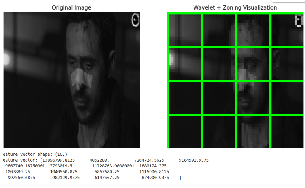
Tackling handwritten mathematical symbols is like deciphering a cryptic code, but the wavelet and zoning hybrid method turned this challenge into a triumph. By combining wavelet transforms for frequency and scale analysis with zoning for localized feature extraction, this approach captures the complexity of variable symbols with elegance.
- Why It’s a Hidden Gem: This hybrid is a niche player in document analysis and optical character recognition (OCR), rarely featured in mainstream machine learning curricula. Its ability to blend statistical and geometrical properties is a unique strength.
- My Application: Applying it to a database of handwritten math equations, I observed superior accuracy compared to standalone wavelet or zoning methods. The method’s ability to handle variability was a highlight of my OCR experiments.
- Academic Insight: Research validates its efficacy, noting improved performance on medium-sized databases due to its comprehensive feature capture (ResearchGate, 2024).
import cv2
import pywt
import numpy as np
import matplotlib.pyplot as plt

def wavelet_zoning_features_with_visualization(image, wavelet='haar', level=2, zones=(4, 4)):
    # Step 1: Apply wavelet transform
    coeffs = pywt.wavedec2(image, wavelet=wavelet, level=level)
    cA = coeffs[0]

    # Step 2: Zoning
    zone_rows, zone_cols = zones
    zone_height = cA.shape[0] // zone_rows
    zone_width = cA.shape[1] // zone_cols

    features = []

    vis_img = cv2.cvtColor(cv2.resize(image, (cA.shape[1], cA.shape[0])), cv2.COLOR_GRAY2BGR)

    for i in range(zone_rows):
        for j in range(zone_cols):
            y1 = i * zone_height
            y2 = (i + 1) * zone_height
            x1 = j * zone_width
            x2 = (j + 1) * zone_width

            zone = cA[y1:y2, x1:x2]
            energy = np.sum(zone**2)
            features.append(energy)

            # Draw rectangle to visualize the zones
            cv2.rectangle(vis_img, (x1, y1), (x2, y2), (0, 255, 0), 1)

    return np.array(features), vis_img

# Load your uploaded image
image = cv2.imread('/mnt/data/3d0d2b30-9d5f-4080-95d3-889c102665e0.png', cv2.IMREAD_GRAYSCALE)

# Safety check
if image is None:
    raise ValueError("Image not found.")

# Resize (optional, for manageable size)
image = cv2.resize(image, (256, 256))

# Extract features and get visualization
features, vis_img = wavelet_zoning_features_with_visualization(image, wavelet='db1', level=2, zones=(4, 4))

# Show
plt.figure(figsize=(12, 6))

plt.subplot(1, 2, 1)
plt.imshow(image, cmap='gray')
plt.title('Original Image')
plt.axis('off')

plt.subplot(1, 2, 2)
plt.imshow(cv2.cvtColor(vis_img, cv2.COLOR_BGR2RGB))
plt.title('Wavelet + Zoning Visualization')
plt.axis('off')

plt.show()

print("Feature vector shape:", features.shape)
print("Feature vector:", features)
Reflections on My Journey
These five methods have not only enhanced my research but also deepened my appreciation for the ingenuity of domain-specific feature extraction. Their “secret” status stems from their confinement to specialized fields like biometrics, forensics, and OCR, where they address challenges that standard techniques struggle with. Each method has taught me the value of looking beyond conventional approaches, inspiring me to explore the fringes of machine learning research.
Key References
Leave a Reply